3.3.1 Rapid Prototyping:
Getting Started

This example shows how to build a simple signal
flow graph to measure energy and then use the results
of the graph to extract energy features.
The steps to create the signal flow graph include:
- I/O:
Learn how to configure a signal flow graph to accept
external data by configuring the transform builder components named
Input and Output.
- Algorithms:
Learn how to create and configure specific algorithm components.
- Graph Manipulation:
Learn how to insert and delete arcs and perform other graph
manipulations.
- Transformations:
Once you have completed the steps to build a signal flow
graph, you will perform the actual feature extraction process
by executing isip_transform.
- Verification:
Learn how to verify the results produced by the example described
above.
In addition to this tutorial, our
workshop notes
contain useful examples of how to perform feature extraction using
our software.
|

|
Configuring I/O:
To begin this phase of the tutorial run transform builder
by executing the command isip_transform_builder.
Next, follow these steps to create the Input and Output components
in your workspace:
|
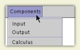
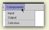
Step 1: In the main panel, click Components and select Input.
|
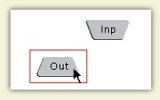
Step 2: Add the Input component to the workspace by clicking in the
white area. Repeat Step 1 for the Output component and place
it in the workspace as well.
|
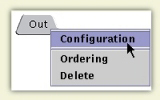
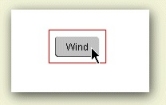
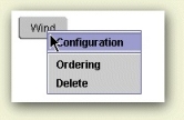
Step 3: After placing the Input and Output components, right
click on the input component and select Configuration from the
popup menu. Configure the parameters for the
Input
component. Repeat this process for the
Output
component.
|
|
|
|
Make sure that implementation in your Output
box is set to "Features." This will direct
isip_transform to output feature vectors.
|
Selecting Algorithm Components:
Placing the Algorithm components is much like placing the Input
and Output components.
|
Step 1: In the main panel, click Components and select the
Window component.
|
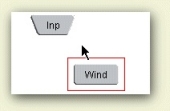
Step 2: Add the Algorithm component to the workspace by clicking
in the white area of the window. Repeat steps one and two for the
Energy component. |
Step 3: After placing the Algorithm component, right click on it and
click Configuration in the pop-up menu. Configure the
parameters for the
Window
component. Repeat this process for the
Energy
component.
|
|
|
|
|
Graph Manipulation:
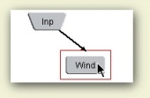
Once the Input, Output, and Algorithm components are placed,
connect them using arcs.
|
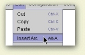
Step 1: From the Edit menu select Insert Arc.
|
Step 2: Connect two components with an arc by selecting
one component and then selecting another component. An arc will
appear, connecting the two Algorithm components. Continue this step
until all the necessary components are connected in the
correct order.
|
Step 3: If you make a mistake, an arc can easily be
deleted. To delete an arc, click Edit in the main panel,
then Delete Arc. Click on the arc (the actual line connecting the
components). Now the arc will disappear.
|
|
|
|
|
Transformations:
Your completed signal flow graph should look similar to the one
on the right of this page.
Now you need to save the signal flow graph to an Sof file.
To save the file, select Save As from the File menu. A
dialog box will pop up. Go to
the directory $ISIP_TUTORIAL/sections/s03/s03_03_p01. Name the file
recipe_energy.sof and then click Save.
Click here
to download an example result.

The following command extracts the features configured in recipe_energy.sof
from speech.sof. Run this command in the directory
$ISIP_TUTORIAL/sections/s03/s03_03_p01.
This command stores the energy measurements in a file named
speech_energy.sof. (Note: If the file speech_energy.sof already
exists, the file will be named speech_energy_n.sof where n
indicates the number of occurrences of the file in the current
directory.)
Click here
to see an example result for this command.
Note the format of the file. The top portion contains
header information from the configuration, such as number
of features extracted, frame duration, and sample frequency.
The data values are shown in the latter part of the file.
Since Sof files are text files, you may view them from any
text editor or software which displays text.
You may also compare your feature file, speech_energy.sof, to the
example results using the diff command, at a Unix command line as
shown:
diff speech_energy.sof ./compare/speech_energy_compare.sof
See Unix on-line manual pages for further details on diff.
(Note: there may be small differences in significance of the
numeric values due to architectural differences in the computer
you are using and the one on which the example features file was
produced.)
For more information on isip_transform proceed to the
next section.
|
Configuring An Input Component:
")
|
Audio Front End Configuration:
- input_data_type: either sampled data or features.
For this example select SAMPLED_DATA.
- data_mode: select FRAME_BASED.
- frame_duration: the duration in seconds
of each data frame, accept the default value, 10 ms.
- signal_duration: not used in this example,
accept default value of 0.1
Click the configure button to the left to configure the
dialog below.
|
SubInput Configuration:
- audio_input: Click the Audio button to the right
to configure Audio_Input. The configuration window below will
open.
|
")
|
")
|
Audio Input Configuration:
- sample_frequency: units are Hz, accept the default
value of 8000.
- file_type: options include binary data or text. Select
BINARY since in this example we are inputing a
binary audio file.
- file_format: options include SOF, RAW, WAV, or SHPERE.
Select SOF.
- byte_order: select LITTLE_ENDIAN.
machine architecture
- compression_type: select LINEAR.
- sample_precision: select NONE.
- sample_num_bytes: accept default value of 2..
- num_channels: since provided file is mono select 1.
- amplitude_range: defines the amplitude range multiplier,
accept the default value of 1.
|
|
Configuring An Output Component:
Note: Configure your Output component as shown in this example.
")
|
Output Configuration:
- algorithm: data is currently the only option supported.
- implementation: options include FEATURES or SAMPLED_DATA;
select FEATURES.
|
SubOutput Configuration:
- feature_output: click on the Feature button to the
right for the Feature configuration dialog.
- file_extension: enter Sof the default format.
- data_mode: options include SAMPLE_BASED or FRAME_BASED;
select FRAME_BASED.
- debug_level: options include NONE, BRIEF, DETAILED, or
ALL; select NONE.
|
")
|
")
|
Feature Output Configuration:
- file_type: option include TEXT or BINARY; select TEXT.
- file_format: options include SOF, or RAW; select SOF.
- compression_type: defines the compression type
of the output file; select the default, LINEAR.
- num_channels: defines the number of channels.
Enter the default value which is 1.
- amplitude_range: defines the amplitude range multiplier;
accept defualt of 1.
|
|
Configuring An Energy Component:
Note: Configure your Energy component as shown in this example.
")
|
Output Configuration:
- algorithm: choices are either SUM or FILTER; select SUM.
- implementation: defines the scaling mode to be used;
select LOG.
|
SubEnergy Configuration:
- floor: limits the minimum value of energy (useful
when performing log operations).
- debug_level: select NONE.
|
")
|
|
Configuring A Window Component:
Note: Configure your Window component as shown in this example.
")
|
Window Configuration:
- algorithm: defines the window functions;
select RECTANGULAR.
- implementation MULTIPLICATION is currently
the only supported option.
|
SubWindow Configuration:
- constants: used to override the default constant values;
leave blank.
- alignment: controls the alignment of the window
with respect to the frame; select LEFT.
- normalization: select NONE.
- compute_mode: select CROSS_FRAME since the window of data
extends outside the current frame.
- duration: defines the duration or length of the windows,
units in seconds.
- debug_level: select NONE.
|
")
|
|


